Hello everyone,
When implementing low-pass filters for the development of an application for my department, an error occurs that I cannot solve.
The goal is the low-pass filtering of acceleration measurements (Nx4 array: time + 3-axis). The filter should be a 4th order Butterworth filter with the cut-off frequency fc.
I have implemented it like this:
fs_n = fs/2 #normalized signal frequency
fc_n = fc/fs_n #normalized cut-off frequency
b, a = signal.butter(order, fc_n, btype=“low”, analog=False)
data_flt = signal.filtfilt(b, a, data)
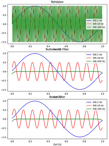
When i create a signal for testing, with a frequency f equals the cut-off frequency fc, the damping of the signal is 0.5 and not 0.707.
Further more the Damping of a Signal with a frequency of 10*fc is ~1/100 and not ~1/10.
Furthermore the signal.butter and the signal.bessel functions deliver the same parameters b and a for the same parameters order, and fc_n. which should not be correct in my understanding - since the frequencyresponses are different.
Following my complete code for testing. There I have generated 3 signals for comparison. One with f = 1/10fc, one with f=fc and one with 10fc. Then i filter the datasets with butter and also with bessel. In the end I compre the results in 3 plots (raw, butter and bessel):
#raw data
dur = 1 #duration
fs = 10000 #frequency of the data signal
f1 = 1
f2 = 10
f3 = 100
nMea = dur*fs #number of measuring points
#base data for filters
fc = 10
order = 1
fig1 = plt.figure(1)
#creating raw data
dataraw = np.zeros((nMea,4)) #Initializing array
dataraw[:,0] = np.linspace(0,dur,int(fsdur),endpoint=False) #time data
dataraw[:,1] = np.sin(2np.pif1dataraw[:,0]) #1 Hz data
dataraw[:,2] = np.sin(2np.pif2dataraw[:,0]) #10 Hz data
dataraw[:,3] = np.sin(2np.pif3dataraw[:,0]) #100 Hz data
#rohdaten anzeigen
ax1 = fig1.add_subplot(311)
ax1.plot(dataraw[:,0], copy.deepcopy(dataraw[:,1]), label='SIN ’ + str(f1) + " Hz",color=“b”)
ax1.plot(dataraw[:,0], copy.deepcopy(dataraw[:,2]), label='SIN ’ + str(f2) + " Hz",color=“r”)
ax1.plot(dataraw[:,0], copy.deepcopy(dataraw[:,3]), label='SIN ’ + str(f3) + " Hz",color=“g”)
ax1.set_title(“Rohdaten”)
ax1.set_xlabel(“Zeit [s]”)
ax1.legend()
#Butter
fs_n = fs/2
fc_n = fc/fs_n
b, a = signal.butter(order, fc_n, btype=“low”, analog=False)
#filter data
data1 = np.zeros((nMea,3))
data1[:,0] = signal.filtfilt(b, a, copy.deepcopy(dataraw[:,1]))
data1[:,1] = signal.filtfilt(b, a, copy.deepcopy(dataraw[:,2]))
data1[:,2] = signal.filtfilt(b, a, copy.deepcopy(dataraw[:,3]))
#showing butter data
ax2 = fig1.add_subplot(312)
ax2.plot(dataraw[:,0], data1[:,0], label='SIN ’ + str(f1) + " Hz",color=“b”)
ax2.plot(dataraw[:,0], data1[:,1], label='SIN ’ + str(f2) + " Hz",color=“r”)
ax2.plot(dataraw[:,0], data1[:,2], label='SIN ’ + str(f3) + " Hz",color=“g”)
ax2.set_title(“Butterworth Filter”)
ax2.set_xlabel(“Time[s]”)
ax2.legend()
#bessel
w2 = fc/(fs/2)
c, d = signal.bessel(order, w2, ‘low’)
#filter data
data2 = np.zeros((nMea,3))
data2[:,0] = signal.filtfilt(c, d, copy.deepcopy(dataraw[:,1]))
data2[:,1] = signal.filtfilt(c, d, copy.deepcopy(dataraw[:,2]))
data2[:,2] = signal.filtfilt(c, d, copy.deepcopy(dataraw[:,3]))
#showing besselfilter data
ax3 = fig1.add_subplot(313)
ax3.plot(dataraw[:,0], data2[:,0], label='SIN ’ + str(f1) + " Hz",color=“b”)
ax3.plot(dataraw[:,0], data2[:,1], label='SIN ’ + str(f2) + " Hz",color=“r”)
ax3.plot(dataraw[:,0], data2[:,2], label='SIN ’ + str(f3) + " Hz",color=“g”)
ax3.set_title(“Bessel Filter”)
ax3.set_xlabel(“Time[s]”)
ax3.legend()
#showing plots
plt.show(block=True)
Here are the plots i get:
Any ideas where the mistake is?
Further Information:
- the comments in my code are in an other language and were translated for this post
- i use the copy.deepcopy method because i wanted to avoid problems with references. I know it is not nessecary
