I’m currently working on a project that aims to enhance scipy’s solve_ivp methods for differential algebraic equations (DAE’s) or implicit differential equations (IDE’s). Specifically, I’m implementing a similar submodule _dae that implements a solve_dae function. Currently, I focus on BDF/ NDF methods and the family of Radau IIA methods. Later I’m planing to add the TR-BDF2 method as well. The current status of this project can be found in my github repository, which mimics the module structure of scipy such that I can easily create a PR later.
Now to my question. Is the scipy community interested in such a feature? Since these methods are purely implemented in python there are no license restrictions at all. Most of the methods are well known in literature and definitely would leverage the potential of scipy’s integrate functionality. I’m focusing on DAE’s with differentiation index 1. For such systems the methods are well behaved (at least in theory) and consistent initial conditions can be computed quite efficient. I’m constantly adding new examples that demonstrate the efficiency of these methods across various scientific disciplines.
The standard approach to deal with higher index DAE’s is that the algebraic components of the error estimate are multiplied by the step-size * max(0, index - 1). Hence, errors of higher index algebraic equations are basically suppressed with decreasing step-size. If this is a desired feature I can easily add this to the implemented methods too.
I’m happy to answer your questions/ start a discussion on this topic here.
Indeed, that formed the basis of this repository. But it relies on the old Hairer & Wanner codes that assume a system of the form My' = f(t, y). More recently (1998), de Swart and Lioen proposed Runge Kutta methods for implicit systems of the form F(t, y, y') = 0. This approach is applied in this repository for the Radau IIA methods with arbitrary number of odd stages and the BDF/ BDF methods of Shampine with quasi constant step-size. For ODE’s this introduces a little overhead but overall is much more general.
I think this would be a good addition to SciPy. The main missing information to maybe trigger the activity is to have some benchmarking with seriously hard problems. How much we can solve, is there a way to compare it to state-of-art etc. is very valuable.
The performance is not as important as correctness at this stage hence it should be mostly about functionality. I think the most straightforward code is the most maintainable and most acceleratable(?!) by rewriting in lower level machinery.
Then we can arrange the remaining rituals of code quality checks, testing coverage etc. It is not smooth sailing as we figure things out late down the line and this might cause frustration hence I don’t want to kill any enthusiasm prematurely by code related issues.
Thanks, @JonasBreuling. This is definitely a gap in SciPy’s functionality. I agree with @ilayn about making sure we have some benchmarks, it would be interesting to know how the methods you propose to add compare to IDA (which you can use in Python using CASADI and DifferentialEquations.jl
@ilayn and @j-bowhay, I totally agree with you that this needs some proper benchmarking. I’m aware the Test Set for IVP Solvers that could be a good starting point. I think I will focus on the Roberson problem, because it is already implemented by most DAE solvers out there.
@j-bowhay I’ve tried to use the CASADI and DifferentialEquations.jl wrapper for IDA. I could solve the Roberson problem with ease, but for CASADI it is hard to get insights into the solver’s stats. When using DifferentialEquations.jl via diffeqpy, the results seem to be very bad. The runtime is way to long due to python/Julia interactions. Moreover, the IDA solver requires way to much function/ Jacobian evaluations. I’ve had a look at sundials IDA documentation and also solve the problem with the most recent sundials version which gave me the following results (rtol=atol=1e-8):
Residual evaluations: 1153
Jacobian evaluations: 93
Compared with the proposed Radau IIA implementation (rtol=atol=1e-8):
stages = 3:
Residual evaluations: 3325
Jacobian evaluations: 131
stages = 5:
Residual evaluations: 2676
Jacobian evaluations: 124
stages = 7:
Residual evaluations: 2817
Jacobian evaluations: 81
Compared with the proposed quasi-constant NDF method (rtol=atol=1e-8):
Residual evaluations: 2082
Jacobian evaluations: 32
Typically, a work-precision comparison is made between different solvers by computing a very accurate solution by choosing, e.g., atol=rtol=1e-19 and comparing the individual methods with different decreasing values for atol, rtol. Since not all methods can easily be accessed in Python I’m not sure how this can be done in a proper way.
Do you have any suggestions how to create the benchmarks?
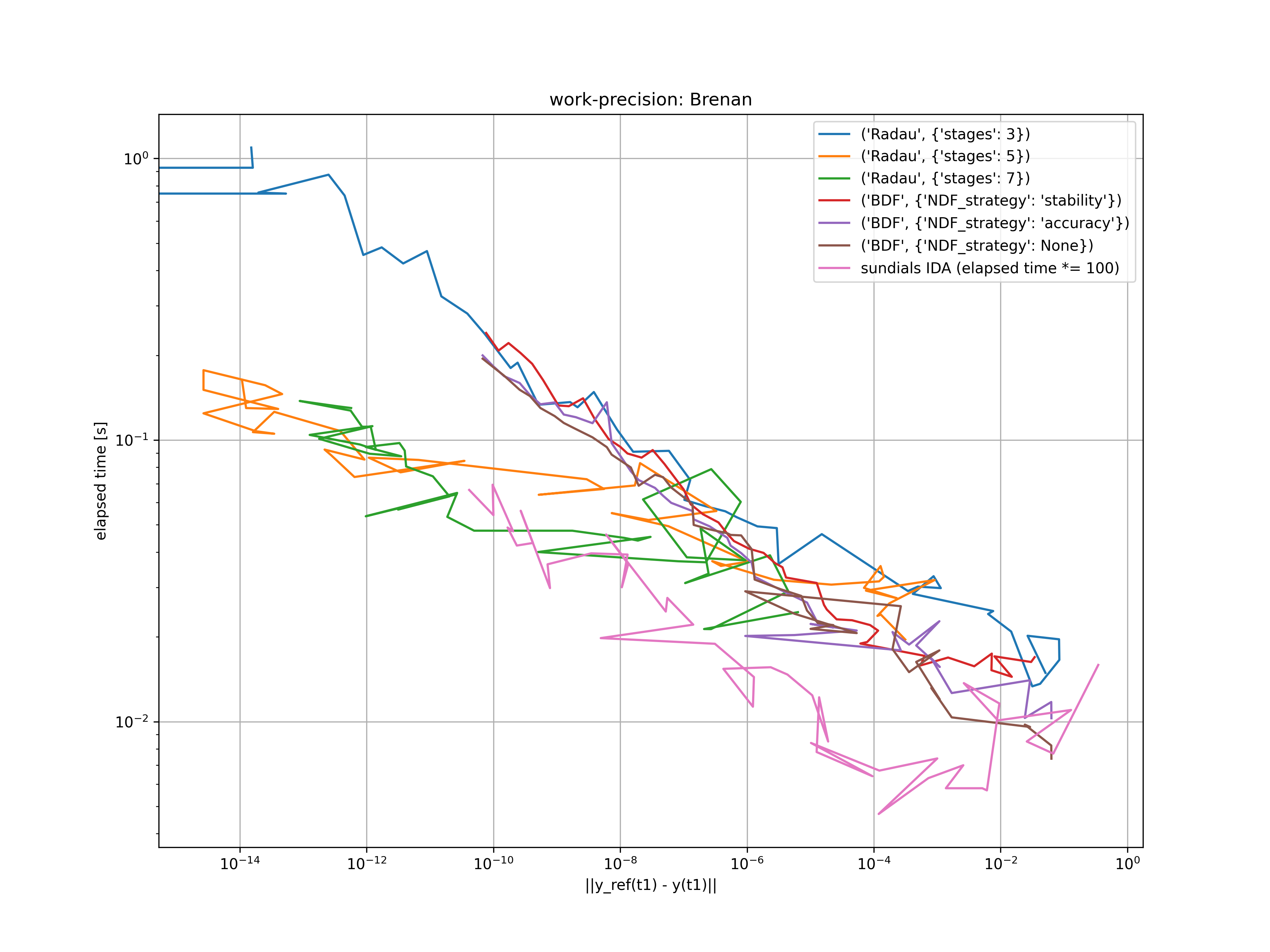
I’ve started creating a simple benchmark procedure. Since I distrust the procedure of using a “very exact” reference solution, I have chosen an index 1 problem which has a known analytical solution. The problem is introduced in the Chapter 4 of the book of Brenan, Campbell and Petzold.
The problem is described by the system of differential algebraic equations
For the consistent initial conditions t_0 = 0, y_1(t_0) = 1, y_2(t_0) = 0, \dot{y}_1 = -1 and \dot{y}_2 = 1, the analytical solution is given by y_1(t) = e^{-t} + t \sin(t) and y_2(t) = \sin(t).
This problem is solved for atol = rtol = 10^{-(1 + m / 4)}, where m = 0, \dots, 45. The resulting error at t_1 = 10 is compared with the elapsed time in the figure below. For reference, the work-precision diagram of sundials IDA solver is also added. Note that the elapsed time is scaled by a factor of 100 since the sundials C-code is ways faster. The source code for the benchmark and the sundials IDA C-code can be found on the main branch of my repository.
Clearly, the family of Radau IIA methods outplay the BDF/NDF methods for low tolerances. For high tolerances, both methods are appropriate. Moreover, the BDF/NDF methods seem to obtain the same accuracy compared to IDA when atol and rtol are chosen the same. I think this is a very satisfactory result. Probably, we should add a scipy benchmark repository somewhere too.
What do you think about these results? I try to implement a similar diagram for the Robertson problem within the next days.
I’v used the sundials C-code and implemented the corresponding example. The C-file as well as a CMakeLists.txt are included to the repository.
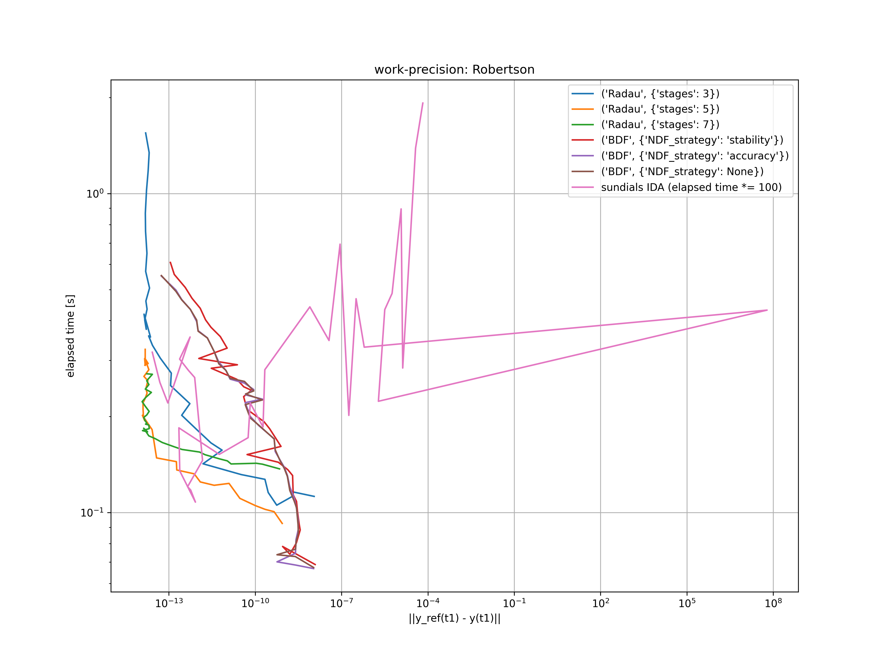
For the Robertson problem the situation is not that easy since it has no analytical solution. I’ve used the values from rober.pdf. The problem is solved for atol = rtol = 10^{-(5.5 + m / 4)}, where m = 0, \dots, 32. The resulting error at t_1 = 1e11 is compared with the elapsed time in the figure below.
Since all three Radau IIA methods and IDA show saturation, the reference solution is probably not accurate enough. Moreover, I’m still confused by the IDA result for smaller tolerances. The relatively large runtimes for large tolerances might be explained by repeated Newton iteration failures, but this is just a guess.
A lot changed until the last time. The repository can now be considered as stable. I’ve added examples with closed form solutions for index 1, 2 and 3 DAEs as well as implicit differential equations. Since the implemented methods only support index 1 DAEs an analytic index reduction is performed.
Probably the last missing piece is adding support for higher-index DAEs. This is classically done by scaling the residual of the index 2 equations by the step-size and the index 3 equations by the step-size**2 to ensure convergence of the Newton iterations. This works for most of the problems but generally leads to more unstable method compared to the analytical index reduction. I think this can be postponed to another pull request, since the changes are very simple but it gives the user a false impression that higher-index problems can solved by the methods without any issues.
If there are further concerns, I will prepare a pull request during the next weeks.